Robotics

Helper page for the Peter Corke: Introduction to robotics MOOC.

Obsah

1 L1 Introduction
2 L2 Position in 2D
3 L3.10 2-axis representation
4 L3.12 Quaternions

L1 Introduction

L2 Position in 2D

Let's create a 2 dimensional rotation matrix for a certain rotation.

 rot2(0)          % zero rotation
 R = rot2(pi/2)   % pi/2 radian rotation stored in R matrix
 rot2(30,'deg')   % rotation 30 degrees
 
 c1 = R(:,1)      % first column of the R
 c2 = R(:,2)      % second column of R

 dot(c1,c2)       % dot product of two vectors
 ans = 0   lebo su pravouhle

 det(R)           % determinant
 ans = 1   lebo su ortogonalne

 inv(R)           % inverse matrix
 R'               % transposition 
                  % mali by byt rovnake
 
 trplot2(R)       % plot the rotated coordination frame
 
 transl2(1,2)     % creates HOMOGENOUS Transformation matrix for translation 
 rot2(30, 'deg')  % creates Rotation matrix
 trot2(30, 'deg') % homogeneous transformation matrix equivalent to the two dimensional rotation matrix 
 
 transl2(1,2) * trot2(30, 'deg') % homogenous matrix consisting of both the rotational and translational parts
 
 se2(1, 2, 30, 'deg')  % omogenous matrix with both rotational and translation parts can be created directly
 
 axis([0 5 0 5]) 
 axis square 
 hold on 
 
 T1 = se2(1, 2, 30, 'deg')
 trplot2(T1, 'frame', '1', 'color', 'b') 
 
 T2 = se2(2,1,0)
 trplot2(T2, 'frame', '2', 'color', 'r')

 T3 = T1 * T2 
 trplot2(T3, 'frame', '3', 'color', 'g') 

 T4 = T2 * T1 
 trplot2(T4, 'frame', '4', 'color', 'c') 
 
 P = [3 2]'   % Create a point using the following notation
 plot_point(P, '*')

 % To determine the coordinate of the point with respect to coordinate frame one, 
 % use the inverse of the relative pose 1 and multiply it by the points coordinate 
 % in the homogeneous form (by appending a 1 to the vector P).
 P1 = inv(T1) * [P ; 1]

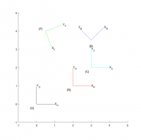
Nakreslime obrazok podobny tomu v prednaske

 axis([-1 5 -1 5]) 
 axis square 
 hold on 

 T0 = se2(0, 0, 0, 'deg')
 trplot2(T0, 'frame', 'O', 'color', 'k') 
 
 T1 = se2(2,1,0)
 trplot2(T1, 'frame', 'R', 'color', 'r')

 T2 = se2(3,2,0)
 trplot2(T2, 'frame', 'C', 'color', 'c')
 
 T3 = se2(3,3.5,45,'deg')
 trplot2(T3, 'frame', 'B', 'color', 'b')

 T4 = se2(0.5,4,-70,'deg')
 trplot2(T4, 'frame', 'F', 'color', 'g')

 T4 =

    0.3420    0.9397    0.5000
   -0.9397    0.3420    4.0000
         0         0    1.0000

Vysledok

Exercise

% DO NOT CHANGE THE FOLLOWING LINES
PA_0 = [6.5; 4.3];  % point A with respect to {0}
PB_2 = [1.2; -2.7];  % point B with respect to {2}

% Modify the following lines to return the correct values
R1 = 
T1 = 
T2 = 
PA_2 = 
PB_1 = 
D_AB =

1. Compute an SO(2) rotation matrix that corresponds to a rotation of -50 degrees and place the result in the workspace variable R1.

R1 = rot2(-50, 'deg');

2. Compute an SE(2) homogenous transformation matrix that corresponds to a translation of 4 in the y-direction and 3 in the x-direction. Place the result in the workspace variable T1.

T1 = transl2(3, 4); % or e.g.:
T1 = se2(3,4,0);

3. Compute an SE(2) homogenous transformation matrix that corresponds to a translation of 5 in the x-direction and 6 in the y-direction and then a rotation of -30 degrees. Place the result in the workspace variable T2.

T2 = se2(5,6,-30,'deg');

4. Consider now that T2 represents the pose of the coordinate frame {2}. The coordinate of point A in the world {0} coordinate frame is given by the workspace variable PA_0. Determine the coordinate of the point with respect to frame {2} and place the result in the workspace variable PA_2.

5. Consider now that T1 represents the pose of the coordinate frame {1}. The coordinate of point B with respect to frame {2} is given by the workspace variable PB_2. 6. Determine the coordinate of point B with respect to the coordinate frame {1}, and place the result in the workspace variable PB_1. 7. Determine the Euclidean distance between point A and point B and place the result in the workspace variable D_AB.

L3.10 2-axis representation

Check understanding: The rotation matrix

 0.9363 −0.2896  0.1987
 0.3130  0.9447 −0.0978
−0.1593  0.1538  0.9752

is equivalent to the 2-vector representation:

A=(−1.8833,6.1427,1.0000),O=(1.0000,−0.4925,4.9085)
A=(1.0000,−0.4925,4.9085),O=(2.9914,1.0000,−0.5091)
A=(1.0000,−0.4925,4.9085),O=(−1.8833,6.1427,1.0000) (CORRECT)
A=(−1.8833,6.1427,1.0000),O=(2.9914,1.0000,−0.5091)

Solution:

o=[-1.8833, 6.1427, 1.0000];     %Orientation vector
a=[1.0000, -0.4925, 4.9085];     %Approach vector
R=oa2r(o,a)    %To create rotation matrix R from o and a vectors

R =

 0.9363         -0.2896         0.1987
 0.3130          0.9447        -0.0978
-0.1593         0.1538         0.9752
 
n=cross(o,a)     %To calculate normal vector n
n =
30.6439       10.2442       -5.2152

r=[n' o' a']     %To create rotation matrix r with columns of n, o, a vectors

# Wrong, n, o and a are unit vectors: 

r=[unit(n') unit(o') unit(a')]     %To create rotation matrix r with columns of n, o, a vectors

tr2rpy(R)     %To calculate roll, pitch and yaw angles from rotation matrix R
tr2rpy(r)     %To calculate roll, pitch and yaw angles from rotation matrix r

Can you please explain:

1. How can matrices R=oa2r(o,a) and r=[n' o' a'] proved to be equivalent? 2. Why is a difference appearing in the yaw angle calculated from matrix R and from matrix r?

Explanation

We can really only do this by trial error, try each of the potential answers and see if it gives the desired rotation matrix. Note that the arguments to the oa2r() function are given in the order O then A, the reverse of what's above.

>> oa2r( [1.0000,   -0.4925,  4.9085], [-1.8833,  6.1427, 1.0000])
>> oa2r( [2.9914, 1.0000,  -0.5091], [1.0000,   -0.4925,  4.9085])
>> oa2r( [-1.8833,  6.1427, 1.0000], [1.0000,   -0.4925,  4.9085])
>> oa2r( [2.9914, 1.0000,  -0.5091], [-1.8833,  6.1427, 1.0000])

L3.12 Quaternions